3D Coordinates

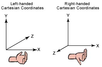
In our project, we use right-hand cartesian coordinates.

However, in computer graphics, we prefer 3D Homogeneous coordinates. This system allows for the representation of points at infinity and simplified equations involving linear transformations. In 3D, a points will represented by a 4 element vector(vec4) $[x,y,z,w]^T$.

The primary benefit of using homogeneous coordinates is that they enable affine transformations (translation, rotation, scaling) and perspective projections to be represented as matrix multiplications. This unifies the handling of different geometric transformations and simplifies the implementation of these operations in computer graphics algorithms. The w does not have a direct physical meaning like x,y,z, its more playing a mathematical role. It is indispensable for the computational and conceptual framework that underpins projective geometry, enabling the representation and manipulation of geometric information in ways that are not possible with only Cartesian coordinates.

Point & Vector

We use vec4 to represent points. In rust, we can use nalgebra-glm, its based on nalgebra, but all APIs are translated in form of GLM in C++. So we can focus on CG math instead of entire Abstract Algebra.

To create a point, its very simple (Note, in our GLM, vectors are COLUMN_MAJOR)

let origin_vec:Vec4 = Vec4::new(0f32,0f32,0f32,1f32);

$$\mathbf{v} = \begin{bmatrix} 0 \cr 0 \cr 0 \cr 1 \end{bmatrix}$$

In fact, a point is no different with vector, however, we would love to use Vec4 $[a,b,c,0]$.

For a point, we are concerned with its coordinate position. However, for a vector, it represents a direction; therefore, a vector does not have a fixed start and end point. We are interested in its direction and magnitude, which often leads to it being decomposed into a unit vector $\mathbf{\hat{v}}$ representing direction (or coefficients of three orthogonal unit vectors) and its magnitude Scala $||\mathbf{v}||$.

Addition, Subtraction, Dot Product, Cross Product and Magnitude & Normalize. The last two is reflection and refraction, its too complicated so we just need to know they are exist.

    let v1:Vec3 = vec3(1.0, 2.0, 3.0);
    let v2:Vec3 = vec3(4.0, 5.0, 6.0);
    
    let add = v1+v2;
    let sub = v1-v2;
	let mult = v1 * 2f32;
    let dot = dot(&v1, &v2);
    let cross = cross(&v1, &v2);
    let mag = magnitude(&v1);
    let norm = normalize(&v1);

$$\mathbf{a} + \mathbf{b} = \begin{bmatrix} a_1 \cr a_2 \cr a_3 \end{bmatrix}+ \begin{bmatrix} b_1 \cr b_2 \cr b_3 \end{bmatrix}= \begin{bmatrix} a_1 + b_1 \cr a_2 + b_2 \cr a_3 + b_3 \end{bmatrix}$$ $$\mathbf{a} - \mathbf{b} = \begin{bmatrix} a_1 \cr a_2 \cr a_3 \end{bmatrix}- \begin{bmatrix} b_1 \cr b_2 \cr b_3 \end{bmatrix}= \begin{bmatrix} a_1 - b_1 \cr a_2 - b_2 \cr a_3 - b_3 \end{bmatrix}$$ $$\mathbf{a} * c = \begin{bmatrix} a_1c \cr a_2c \cr a_3c \end{bmatrix}$$ $$\mathbf{a} \cdot \mathbf{b} = \begin{bmatrix} a_1 & a_2 & a_3 & a_4 \end{bmatrix} \cdot \begin{bmatrix} b_1 \cr b_2 \cr b_3 \cr b_4 \end{bmatrix}= a_1b_1 + a_2b_2 + a_3b_3 + a_4b_4$$ $$\mathbf{a} \times \mathbf{b} = \begin{bmatrix} 0 & -a_3 & a_2 \cr a_3 & 0 & -a_1 \cr -a_2 & a_1 & 0 \end{bmatrix} \begin{bmatrix} b_1 \cr b_2 \cr b_3 \end{bmatrix} = \begin{bmatrix} -a_3b_2 + a_2b_3 \cr a_3b_1 - a_1b_3 \cr -a_2b_1 + a_1b_2 \end{bmatrix}$$ $$\|\mathbf{v}\| = \sqrt{v_1^2 + v_2^2 + v_3^2}$$ $$\mathbf{\hat{v}} = \frac{\mathbf{v}}{||\mathbf{v}||} = \frac{1}{\sqrt{v_1^2 + v_2^2 + v_3^2}} \begin{bmatrix} v_1 \cr v_2 \cr v_3 \end{bmatrix}$$ $$\mathbf{r} = \mathbf{i} - 2(\mathbf{i} \cdot \mathbf{n})\mathbf{n}$$ $$\mathbf{t} = \eta \mathbf{i} + \left(\eta \cos(\theta_i) - \sqrt{1 - \eta^2 \left(1 - \cos^2(\theta_i)\right)} \right) \mathbf{n}$$

Dot Production

Vector add or subtract Vector is still a Vector. But when vector's dot product is a Scala, as we show before: $$\mathbf{a} \cdot \mathbf{b} = \begin{bmatrix} a_1 & a_2 & a_3 & a_4 \end{bmatrix} \cdot \begin{bmatrix} b_1 \cr b_2 \cr b_3 \cr b_4 \end{bmatrix}= a_1b_1 + a_2b_2 + a_3b_3 + a_4b_4\\$$ We can obtain the angle between two vectors by calculating their dot product. $$\mathbf{a} \cdot \mathbf{b} = ||\mathbf{a}|||\mathbf{b}||\cos{\theta}\\$$ $$\cos{\theta} = \mathbf{\hat{a}}\cdot\mathbf{\hat{b}}\\$$ $$\theta = \arccos{(\mathbf{\hat{a}}\cdot\mathbf{\hat{b}})}$$ Vector dot production satisfies the commutative law, associative law, and distributive law. $$\mathbf{a} \cdot \mathbf{b} = \mathbf{b} \cdot \mathbf{a}$$ $$\mathbf{a} \cdot (\mathbf{b} + \mathbf{c}) = \mathbf{a} \cdot \mathbf{b} + \mathbf{a} \cdot \mathbf{c}$$ $$k\mathbf{a} \cdot \mathbf{b} = \mathbf{a} \cdot k\mathbf{b} = k (\mathbf{a} \cdot \mathbf{b})$$

With dot production, we can do Projection (Decomposition) in CG by Gram–Schmidt process:

$$\mathbf{b}_{\perp \mathbf{a}}=||\mathbf{b}\_{\perp \mathbf{a}}||\mathbf{\hat{a}}=||\mathbf{b}||\mathbf{\hat{a}}\cos\theta =\left( \frac{\mathbf{b} \cdot \mathbf{a}}{\|\mathbf{a}\|^2} \right) \mathbf{a}$$

Therefore, we can also decompose any vector into the sum of three orthogonal unit vectors $\mathbf{x}$, $\mathbf{y}$, and $\mathbf{z}$​.

$$\mathbf{p} = (\mathbf{p}\cdot\mathbf{x})\mathbf{x} +(\mathbf{p}\cdot\mathbf{y})\mathbf{y}+(\mathbf{p}\cdot\mathbf{z})\mathbf{z}$$

Through the result of the dot product, we can also determine the relative direction of two vectors. For example, a dot product equal to 0 means orthogonal, a dot product greater than 0 indicates the same direction, and conversely, a negative dot product indicates opposite directions.

Cross Production

The cross product of vectors $\mathbf{a}$ and $\mathbf{b}$ results in a new vector $\mathbf{c}$, which is orthogonal to the plane defined by $\mathbf{a}$ and $\mathbf{b}$, and is known as the normal vector. It's important to note that the order of the cross product determines the direction of the normal vector, and this calculation follows the right-hand rule. $$\mathbf{a} \times \mathbf{b} = \mathbf{A}^*\mathbf{b} = \begin{bmatrix} 0 & -a_3 & a_2 \cr a_3 & 0 & -a_1 \cr -a_2 & a_1 & 0 \end{bmatrix}\begin{bmatrix} b_1 \cr b_2 \cr b_3 \end{bmatrix}= \begin{bmatrix} -a_3b_2 + a_2b_3 \cr a_3b_1 - a_1b_3 \cr -a_2b_1 + a_1b_2 \end{bmatrix}$$ $$||\mathbf{a} \times \mathbf{b}|| = ||\mathbf{a}||||\mathbf{b}||\sin\theta\\$$ The commutative law, associative law, and distributive law will be slightly different. Note, in $\mathbf{a} \times \mathbf{a} = \mathbf{0}$, the $\mathbf{0}$ is still a zero-magnitude vector, not a scalar. $$\mathbf{a} \times \mathbf{b} = -\mathbf{b} \times \mathbf{a}$$ $$\mathbf{a} \times \mathbf{a} = \mathbf{0}$$ $$\mathbf{a} \times (\mathbf{b} + \mathbf{c}) = \mathbf{a} \times \mathbf{b} + \mathbf{a} \times \mathbf{c}\\$$ $$k\mathbf{a} \times \mathbf{b} = \mathbf{a} \times k\mathbf{b} = k (\mathbf{a} \times \mathbf{b})$$ Do you remember what we said about the right-hand coordinate system? Regarding how to define a right-hand coordinate system, it satisfies the condition that the unit orthogonal vectors x cross y equals z, which defines the right-hand coordinate system. $$\mathbf{x} \times \mathbf{y} = \mathbf{z}\\$$ Similar to the dot product, through the cross product of two vectors $\mathbf{a}$ and $\mathbf{b}$, we can determine on which side of $\mathbf{a}$, vector $\mathbf{b}$, lies. For example, when greater than 0, $\mathbf{b}$, is in the counter clockwise direction of $\mathbf{a}$, (left side), and when less than 0, $\mathbf{b}$, is in the clockwise direction of $\mathbf{a}$,(right side). Through this operation, we can determine whether a point P is inside a polygon. We consider the polygon as a series of vectors connected head to tail, and cross each with a vector from a point to P. If all the cross product results have the same sign, this indicates that the point is inside the polygon.

Matrix

We use mat4 to represent a matrix. To generate a unit matrix:

let unit_mat:Mat4 = Mat4::identity();

$$\mathbf{I} = \begin{bmatrix} 1 & 0 & 0 & 0 \cr 0 & 1 & 0 & 0 \cr 0 & 0 & 1 & 0 \cr 0 & 0 & 0 & 1 \end{bmatrix}$$

Matrix transpose (Note, in OpenGL and GLM, mats are COLUMN_MAJOR):

    let natrual_mat = mat4(
        1.0, 2.0, 3.0, 4.0,
        5.0, 6.0, 7.0, 8.0,
        9.0, 10.0, 11.0, 12.0,
        13.0, 14.0, 15.0, 16.0,
    );
    let natrual_mat_t = transpose(&natrual_mat);

$$\mathbf{A} = \begin{bmatrix} 1 & 5 & 9 & 13 \cr 2 & 6 & 10 & 14 \cr 3 & 7 & 11 & 15 \cr 4 & 8 & 12 & 16 \end{bmatrix}$$ $$\mathbf{A}^T = \begin{bmatrix} 1 & 2 & 3 & 4 \cr 5 & 6 & 7 & 8 \cr 9 & 10 & 11 & 12 \cr 13 & 14 & 15 & 16 \end{bmatrix}$$

Addition, Subtraction, Multiplication are overdried already.

    let natrual_mat_add = natrual_mat + natrual_mat_t;
    let natrual_mat_sub = natrual_mat - natrual_mat_t;
    let natrual_mat_mul_vec = natrual_mat * origin_vec;
    let natrual_mat_mul_mat = natrual_mat * natrual_mat_t;

$$\mathbf{A} = \begin{bmatrix} a_{11} & a_{12} & a_{13} & a_{14} \cr a_{21} & a_{22} & a_{23} & a_{24} \cr a_{31} & a_{32} & a_{33} & a_{34} \cr a_{41} & a_{42} & a_{43} & a_{44} \end{bmatrix}, \quad \mathbf{B} = \begin{bmatrix} b_{11} & b_{12} & b_{13} & b_{14} \cr b_{21} & b_{22} & b_{23} & b_{24} \cr b_{31} & b_{32} & b_{33} & b_{34} \cr b_{41} & b_{42} & b_{43} & b_{44} \end{bmatrix},\quad \mathbf{v} = \begin{bmatrix} v_{1} \cr v_{2} \cr v_{3} \cr v_{4} \end{bmatrix}$$ $$\mathbf{A} + \mathbf{B} = \begin{bmatrix} a_{11} + b_{11} & a_{12} + b_{12} & a_{13} + b_{13} & a_{14} + b_{14} \cr a_{21} + b_{21} & a_{22} + b_{22} & a_{23} + b_{23} & a_{24} + b_{24} \cr a_{31} + b_{31} & a_{32} + b_{32} & a_{33} + b_{33} & a_{34} + b_{34} \cr a_{41} + b_{41} & a_{42} + b_{42} & a_{43} + b_{43} & a_{44} + b_{44} \end{bmatrix}$$ $$\mathbf{A} - \mathbf{B} = \begin{bmatrix} a_{11} - b_{11} & a_{12} - b_{12} & a_{13} - b_{13} & a_{14} - b_{14} \cr a_{21} - b_{21} & a_{22} - b_{22} & a_{23} - b_{23} & a_{24} - b_{24} \cr a_{31} - b_{31} & a_{32} - b_{32} & a_{33} - b_{33} & a_{34} - b_{34} \cr a_{41} - b_{41} & a_{42} - b_{42} & a_{43} - b_{43} & a_{44} - b_{44} \end{bmatrix}$$ $$\mathbf{A}\mathbf{v}= \begin{pmatrix} a_{11}v_{1} + a_{12}v_{2} + a_{13}v_{3} + a_{14}v_{4} \cr a_{21}v_{1} + a_{22}v_{2} + a_{23}v_{3} + a_{24}v_{4} \cr a_{31}v_{1} + a_{32}v_{2} + a_{33}v_{3} + a_{34}v_{4} \cr a_{41}v_{1} + a_{42}v_{2} + a_{43}v_{3} + a_{44}v_{4} \end{pmatrix}$$ $$\mathbf{A} \times \mathbf{B} = \begin{pmatrix} \sum_{k=1}^{4} a_{1k}b_{k1} & \sum_{k=1}^{4} a_{1k}b_{k2} & \sum_{k=1}^{4} a_{1k}b_{k3} & \sum_{k=1}^{4} a_{1k}b_{k4} \cr \sum_{k=1}^{4} a_{2k}b_{k1} & \sum_{k=1}^{4} a_{2k}b_{k2} & \sum_{k=1}^{4} a_{2k}b_{k3} & \sum_{k=1}^{4} a_{2k}b_{k4} \cr \sum_{k=1}^{4} a_{3k}b_{k1} & \sum_{k=1}^{4} a_{3k}b_{k2} & \sum_{k=1}^{4} a_{3k}b_{k3} & \sum_{k=1}^{4} a_{3k}b_{k4} \cr \sum_{k=1}^{4} a_{4k}b_{k1} & \sum_{k=1}^{4} a_{4k}b_{k2} & \sum_{k=1}^{4} a_{4k}b_{k3} & \sum_{k=1}^{4} a_{4k}b_{k4} \end{pmatrix}$$

The Mat4 times Mat4, Mat4 times Vec4 still gives us a Mat4, because our Mat have same number of rows and columns.

So in this way, if we want to do some linear transform (Mat4 $\mathbf{A},\mathbf{B},\mathbf{C}$) on our point $\mathbf{v}$, we can do this: $$\mathbf{v'} = \mathbf{A}\times[\mathbf{B}\times[\mathbf{C}\mathbf{v}]] = [\mathbf{A}\times\mathbf{B}\times\mathbf{C}]\mathbf{v}$$ Also we can have inverse (if possible):

let natrual_mat_inv = inverse(&natrual_mat);

$$\mathbf{A}\mathbf{A^{-1}} = \mathbf{A^{-1}}\mathbf{A} = \mathbf{I}$$

in nalgebra-glm, if $\mathbf{A}$ is invertible, its inverse is computed using LU decomposition. For special matrices such as positive definite matrices, Cholesky decomposition is used to accelerate the process. For matrices with a huge condition number, SVD decomposition may be used to improve accuracy in computing the pseudo-inverse, among other numerical methods. If $\mathbf{A}$ is not invertible, it returns None. In computer graphics, we generally do not need to deal with overly complex operations, so there is little need to understand this part in depth, and inverses are rarely used.